Vector Graphics

Introduction

Vector graphics use points, lines, curves, and polygons to construct a scalable image. Try zooming in as much as possible on the figure in this PDF document drawn with vector graphics and prepared in LaTeX. In contrast to raster graphics, notice how you can scale the image to any size without degrading quality.

There are several formats for vector graphics. Some common formats include the Scalable Vector Graphics (SVG) language (also see SVGBasics tutorials), Adobe Illustrator (AI), PostScript (PS), and encapsulated PostScript (EPS). My experience with applications in meteorology leads me to believe that EPS graphics would be the most beneficial to learn about here, but others have had some success with the newer SVG format. Before we begin with EPS, let's start by learning about plain PostScript.

Editing PostScript

Start by downloading applestar.ps onto Blizzard. Type the following at the prompt: gv applestar.ps & If something happens, then you have a program called GhostView in your path and you may skip to the next paragraph. If instead you get gv: Command not found. then you need to make a few changes to your setup. A .cshrc file tells Blizzard which commands to execute when you log in. You can customize your session by adding commands to this file. If you do not already have a .cshrc file in your home directory (test this with ls -la), then type the following commands to retrieve my .cshrc file: cd
wget http://frost.atms.unca.edu/~cgodfrey/advcomp/.cshrc
source .cshrc If you already have a .cshrc file in your home directory (you should!), simply add the commands found in my minimal .cshrc file and source it. Then try gv applestar.ps & again. (Note to UNC Asheville students: The proper commands should already be in your .cshrc file. If not, please contact me.)

Ignore any errors that show up in your terminal window by hitting Enter. Be sure to scroll down in the GhostView window to see the graphic! Now open applestar.ps in a text editor to see the PostScript commands. (If you ever used an Apple IIe, you may notice that the basic idea of drawing with these commands is not that different from Apple Logo.) Now grab applestar.eps and view the file with both GhostView and with a text editor. The only difference between applestar.ps and applestar.eps is that the first line of applestar.ps has been replaced by %!PS-Adobe-3.0 EPSF-3.0
%%BoundingBox: 85 0 475 400 and the showpage command has been removed. The file applestar.eps is an encapsulated PostScript file. The BoundingBox specifies the region beyond which nothing gets rendered and contains the lower-left and upper-right x and y coordinates. You can locate the coordinates for a BoundingBox by moving the cursor in the GhostView window of your .ps file and looking in the top left corner of the GhostView window. Encapsulated PostScript files work beautifully when embedded within document preparation software such as L^aT_eX. The American Meteorological Society prefers EPS formatted figures in manuscripts submitted for publication. You can create or view .eps files in programs such as IDL, Adobe Photoshop, Adobe Illustrator, Inkscape, and several others. Importantly, the Matplotlib library for Python can also create beautiful plots as native .eps files.

Now edit applestar.eps with a text editor and see if you can make something interesting. You can use this Summary of PostScript Commands as a reference. A First Guide to PostScript provides a nice introduction and tutorial. The PostScript tips at Prepressure include help with rendering PostScript and dealing with errors.

Modifying Generated PostScript

Sometimes you may find it useful to modify PostScript output from a program. Let's use a program called gnuplot to accomplish this. At the Linux prompt, try the following: gnuplot
gnuplot> plot cos(x)
gnuplot> set term postscript eps color
gnuplot> set output 'cos.eps'
gnuplot> replot
gnuplot> quit
Use gv cos.eps to view your plot and then open it up in a text editor. Because this is generated output, it's a bit more complicated than applestar.eps. Open cos.eps with a text editor and scroll to the end of the file where you will see lots of lines like 64 -397 V You won't find V in the PostScript tutorials, so what does it mean? Near the top of the file, you will notice that V is defined as a shorthand way to write the "rlineto" command with /V {rlineto} bind def At the top of the file, you will notice that several other shorthand definitions appear here as well. For example, the LT0 command is defined by /LT0 { PL [] 1 0 0 DL } def and describes the RGB colors (1 0 0 or bright red in this case), among other things. Now you can modify your plot in the following ways:

• Change the color of the cosine wave by changing the RGB colors in the LT0 definition
• Comment out the legend with a % symbol
• Adjust the width of your line by inserting 30 setlinewidth right after the second LT0 command.
• Change the font size in the line (Helvetica) findfont 140 scalefont setfont, noting that the font is scaled by 0.050 0.050 scale.
• See what dashed lines look like if you try plot sin(x),cox(x) within gnuplot.

Converting PostScript Graphics to Raster Graphics

You can use ImageMagick to convert your PostScript graphics into raster graphics for display on a Web page: convert applestar.eps applestar_alias.png
convert +antialias applestar.eps applestar_noalias.png Compare the size of your new files with ls -l *.png and then open both images with eog and look at the subtle differences. Note that the +antialias option, described in ImageMagick Command-line Options, actually turns off the antialiasing. Antialiasing softens corner regions by blurring colors a bit and creating the appearance of a smoother transition. The resulting raster image uses more colors and therefore becomes a bit larger.

Plotting METAR Observations

For your assignment, you will create station plots of METAR observations, much like what you would see at RAP Real-Time Weather Data. To simplify things a bit, we will use a Python utility written by Brian Fiedler called "vplot" to write out PostScript commands. Visit vplot to learn all about it and note that simpleSVG replaces vplot, but makes SVG graphics instead of PostScript graphics. For now, we'll use vplot here and I'll make a note to change this someday. Anyway, grab stnplot.tar and untar it with tar xvf stnplot.tar Follow the directions in the README file and look at the comments within stnplot.py. Your finished product might look something like the figure below.

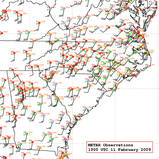Figure 1: Surface map depicting observations at 1900 UTC 11 February 2009. Colors correspond with the extent of cloud cover.

Station Plot Resources

MetarWeather is a nifty (and free) Windows program that downloads and decodes recent METAR observations. Archived raw and decoded observations are also available from Plymouth State. You may use the data file that I included in the assignment, but you could also download and plot your own set of observations. I massaged the decoded METAR reports a bit to produce 200902111900metar.dat for the assignment, so you may need to do the same if you decide to go this route. You can read about METAR code in Surface Weather Observations and Reports. The National Weather Service JetStream - Online School for Weather has a great resource for interpreting surface weather plots, where you can learn how to create a station plot.