Vector GraphicsIntroductionVector graphics use points, lines, curves, and polygons to construct a scalable image. Try zooming in as much as possible on the figure in this PDF document drawn with vector graphics and prepared in LaTeX. In contrast to raster graphics, notice how you can scale the image to any size without degrading quality. There are several formats for vector graphics. Some common formats include the Scalable Vector Graphics (SVG) language (also see SVGBasics tutorials), Adobe Illustrator (AI), PostScript (PS), and encapsulated PostScript (EPS). My experience with applications in meteorology leads me to believe that EPS graphics would be the most beneficial to learn about here, but others have had some success with the newer SVG format. The benefit of SVG is that a browser can render it directly. Let's go ahead and learn about PostScript first and then you can make your own SVG and/or EPS graphics for station plots. Before we begin with EPS, let's start by learning about plain PostScript. Editing PostScriptStart by downloading applestar.ps onto Blizzard. Type the following at the prompt: gv applestar.ps & If something happens, then you have a program called GhostView in your path and you may skip to the next paragraph. If instead you get gv: Command not found. then you need to make a few changes to your setup. A .cshrc file tells Blizzard which commands to execute when you log in. You can customize your session by adding commands to this file. If you do not already have a .cshrc file in your home directory (test this with ls -la), then please contact me for instructions. If you already have a .cshrc file in your home directory (you should!), simply add the path to your gv program and source .cshrc. Then try gv applestar.ps & again. (Note to UNC Asheville students: The proper commands should already be in your .cshrc file. If not, please contact me.)
Ignore any errors that show up in your terminal window by hitting Enter.
Be sure to scroll down in the GhostView window to see the graphic!
Now open applestar.ps in a text editor to see the PostScript commands.
(If you ever used an Apple IIe, you may notice that the basic idea of drawing with these commands is not that different from Apple Logo.)
Now grab applestar.eps and view the file with both GhostView and with a text editor.
The only difference between applestar.ps and applestar.eps is that the first line of applestar.ps has been replaced by
%!PS-Adobe-3.0 EPSF-3.0 Now edit applestar.eps with a text editor and see if you can make something interesting. You can use this Summary of PostScript Commands as a reference. A First Guide to PostScript provides a nice introduction and tutorial. The PostScript tips at Prepressure include help with rendering PostScript and dealing with errors. Modifying Generated PostScript
Sometimes you may find it useful to modify PostScript output from a program.
Let's use a program called gnuplot to accomplish this.
At the Linux prompt, try the following:
gnuplot
Converting PostScript Graphics to Raster Graphics
You can use ImageMagick to convert your PostScript graphics into raster graphics for display on a Web page:
convert applestar.eps applestar_alias.png MetPy and Python 3.xMetPy is a collection of tools in Python that are specific to meteorological applications. I have installed MetPy on Blizzard, but these tools will only work with Python 3. Therefore, I have created a separate Anaconda distribution that we can manage easily. To use this version of Python, add the following line to the end of your .cshrc file located in your home directory: setenv PATH ${PATH}:/usr/local/anaconda3/bin To access Python 3 without logging out and back in again, enter this at the Blizzard prompt: source .cshrc This sources your .cshrc file, which is a list of commands that will run when you first log in. You have just told Blizzard to look in this location for any executable programs. Now you can access the Anaconda distribution of Python 3 with python3 If this opens up a python prompt with Python 3.7.6 (or later), then you're all set! You will notice a few differences between Python 2.x and Python 3.x. As I mentioned in the Python tutorial, the most consequential difference that you may notice is with the syntax of print statements. Plotting METAR Observations
I borrowed much of this code from the Unidata developers, so you will see their comments interspersed with mine. Carefully read the comments within stnplot.py. For credit, make the following changes:
Post your program and your final SVG file to your password-protected Web page. Your finished product might look something like Figure 2 below. Click on the map to see the original SVG image. In your browser, hit Ctrl-+ (Ctrl and the + key) to zoom in. Notice that the elements in the image remain crisp no matter how much you zoom in!
ResourcesYou can read about METAR code in Surface Weather Observations and Reports. The National Weather Service JetStream - Online School for Weather has a great resource for interpreting surface weather plots, where you can learn all about station plots. You will find the Cartography and Mapping in Python tutorial very helpful as you learn to add gridlines and make high-resolution borders and backgrounds. Note that the NASA URL for Web Map Services (WMS) can change, so you may need to visit the top-level NASA URL outlined in this tutorial to find a new WMS URL. Additional information on background layers is in this Exploring What's New in Cartopy tutorial. NCAR has another example showing how to use Matplotlib with Cartopy when working with WRF data. Directions for using the Cartopy Feature Interface may be useful as well. Lastly, Python's datetime module will be helpful as you format the date for your title. Pay particular attention to the strptime() and strftime() functions. For reference, here is the old assignment from 2009–18. |
 |
 |
 |
|
|


 For your assignment, you will create station plots of METAR observations, much like what you would see at
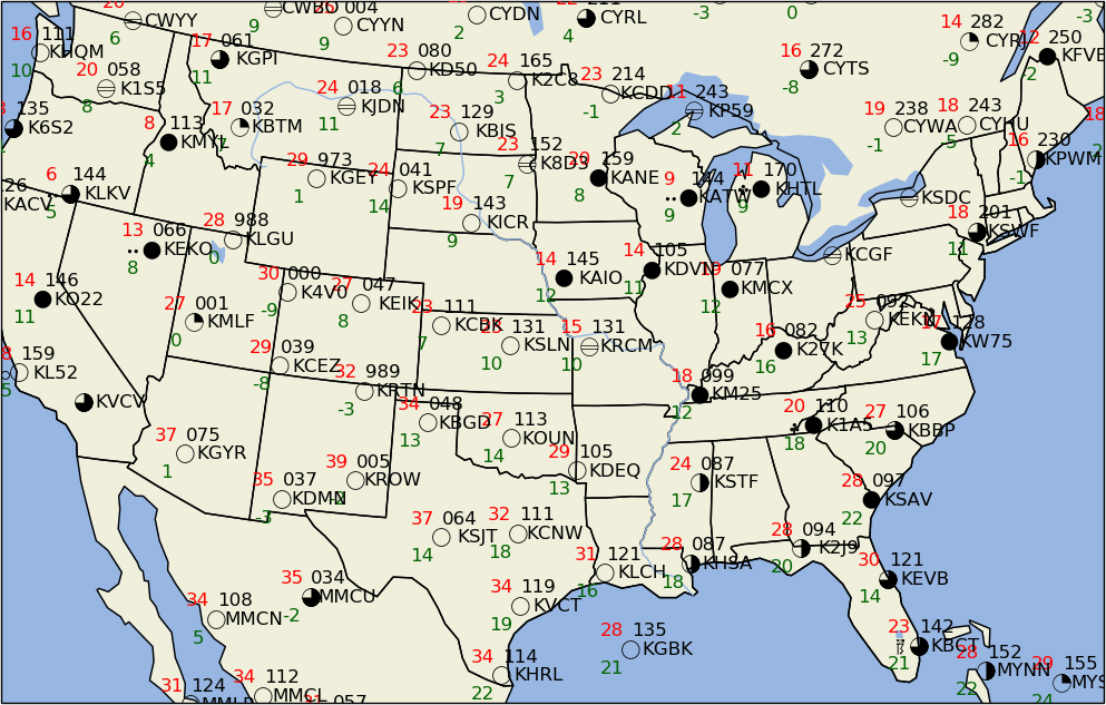

| North Carolina's Public Liberal Arts University |